[Brief Review] Beyond Single Path Integrated Gradients for Reliable Input Attribution via Randomized Path Sampling

Takeaway Summary

Keywords: Integrated Gradients (IG), path integration, XAI, attribution method, path-based attribution method, path sampling, stick-breaking path sampling, Dirichlet Prior

✅ IG constructed by aggregating attributions from the multiple paths: Averaging Integrated Gradients across many sampled trajectories drastically suppresses path‑specific noise, yielding cleaner and more object‑aligned explanations.

✅ Randomized path sampling - Stick-breaking Path Integration: A stick‑breaking process with tunable concentration \(\alpha\) generates a diverse, yet analytically tractable, distribution of integration paths that subsumes the straight‑line IG as a special case.

✅ Statistical visualization with SPI‑P: By converting each pixel’s attribution distribution into the probability it exceeds a top‑5 % threshold, SPI‑P highlights features that contribute consistently and positively across all paths.

Brief Review

Summary

1. Problem Statement
   • Integrated Gradients (IG) integrates along a single straight path, which yields path‑dependent noise and prevents the heat‑map from being well object‑aligned.
   • Even variants such as Guided IG only modify one path and therefore cannot eliminate the variance that arises from using a single trajectory.
2. Main Idea
   • Generate multiple randomized integration paths, compute IG separately for each path, and aggregate their attribution scores. This statistical averaging effectively reduces noise, thereby enhancing the reliability of attribution results.

3. Path Sampling - Stick-Breaking Process (SBP)

   

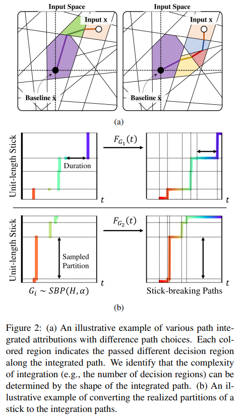
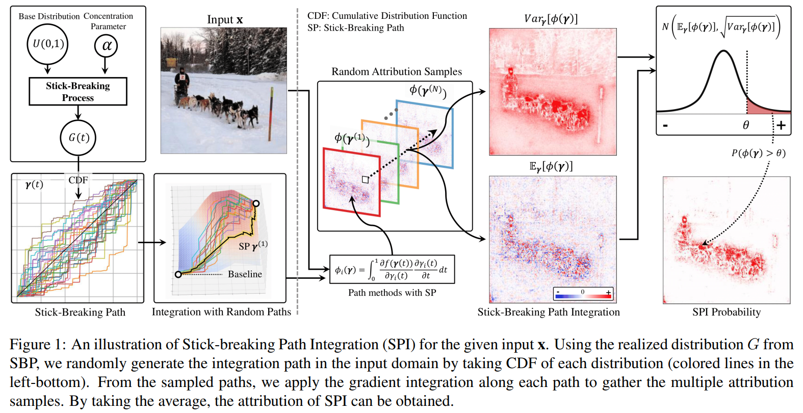
   • Construction: Break a unit stick repeatedly to obtain piece lengths \(\pi_k\) and locations \(t_k\) , then build a probability‑mass function \(\displaystyle G(t)=\sum_k \pi_k ,\delta_{t_k}(t)\) , and use its CDF, \(F_G(t)\) , as the per‑feature integration path.
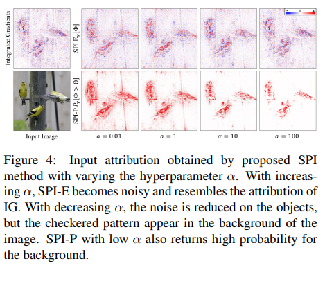
   • Concentration parameter \(\alpha(\beta_k\sim\mathrm{Beta}(1,\alpha))\) : Large \(\alpha\) \(\Rightarrow\) paths converge to the IG straight line (low diversity); small \(\alpha\) \(\Rightarrow\) diverse step‑like paths
4. SPI
   • For a model  \(f\) , an input  \(\mathbf x\) , and a baseline  \(\bar{\mathbf x}\) , let each feature–wise path be driven by a stick‑breaking process \(G_i\sim\text{SBP}(U(0,1),\alpha)\) with CDF  \(F_{G_i}(t)\) . Then the SPI attribution for feature  \(i\) is the expectation of Integrated Gradients over that path distribution:
   \[SPI_i(\mathbf{x}; \alpha) = \mathbb{E}_\gamma[\phi_i(\gamma)] \\ = \mathbb{E}_{G} \left[ (x_i - \bar{x}_i) \int_0^1 \frac{\partial f\left(\bar{\mathbf{x}} + F_G(t) \odot (\mathbf{x} - \bar{\mathbf{x}})\right)}{\partial\left(\bar{x}_i + F_G(t)(x_i - \bar{x}_i)\right)} \frac{dF_G(t)}{dt} \, dt \right]\]
   • inner integral: the standard line integral that defines Integrated Gradients along a specific path determined by \(F_{\mathbf G}(t)\) ;
   • outer expectation: averages those IG values over all SBP‑sampled paths, removing path‑specific noise;
   • \(\alpha\) controls diversity: \(\alpha\uparrow\)   \(\Rightarrow\) paths converge to the straight IG line, \(\alpha\downarrow\)   \(\Rightarrow\) more step‑like variations.
   • Averaging across paths greatly reduces noise and yields more object‑aligned maps
5. SPI-P (Probability)
   • If a pixel’s attribution scores significantly vary across different integration paths, its attribution reliability is low—even if its average attribution is notably high or low. (In contrast, pixels that consistently show high or low attribution with low variance are reliably indicating a stable contribution, demonstrating less sensitivity to the specific integration path.)

   • Model each pixel’s distribution as \(\mathcal N(\mu,\sigma^2)\) and compute the right‑tail probability that it exceeds the 95‑percentile threshold \(\Theta\) (top 5 % of SPI‑E values):

     \[SPI\text{-}P_i(\mathbf{x}; \alpha) = \mathbb{P}(\Phi_i > \Theta) \\= 1 - \frac{1}{\sigma \sqrt{2\pi}} \int_{-\infty}^{\Theta} \exp\left( -\frac{(\theta - \mu)^2}{\sigma^2} \right) d\theta\]
   • Pixels with high \(\text{SPI‑P}\) contribute frequently and stably.
6. Experiments
   • Insertion / Deletion (ImageNet‑val, VGG‑16, Inception‑v3, ResNet‑18): SPI achieves the best area‑under‑curve scores on every model.
   • ROAR (CIFAR‑10, ResNet‑18): removing the top 10 % SPI pixels and retraining causes the largest drop in accuracy, confirming that SPI pin‑points information the model truly relies on.

Overview

• Task: Input attribution based on Integrated Gradients (IG)
• Goal: Obtaining clearer and more reliable input attribution
• Existing Problems
  • The exsiting single path IG methods often produce noisy and unreliable attributions during the integration of the gradients over the path defined in the input space.
• Rationale behind the proposed method:
  • Neural networks with piecewise linear activation functions, such as ReLU, construct piecewise linear decision spaces. To enhance the expressivity of deep neural networks, the number of linear regions has increased. Consequently, applying only a single integration path in path-based attribution methods leads to high uncertainty and variance in the resulting attributions. To mitigate the uncertainty introduced by selecting a single integration path, they propose computing the expectation of the path-based attributions over a distribution of possible paths.
• Contributions:
  • Address the inconsistency in attribution caused by the choice of integration paths.
  • Propose a random sampling method for generating integration paths inspired by the Stick-Breaking Process.
  • Propose an improved visualization method for attribution by leveraging statistical analyses of attribution scores, enabling clearer interpretation.
  • Validate the reliability of the proposed method across various network architectures.
• Limitations & Possible future works:
  • Choosing Alternative Base Distributions:
    • The paper uses a stick-breaking process (SBP) anchored on a uniform base distribution \(H=U(0,1)\) , ensuring the average path matches the linear path used in IG.
    • The authors note that replacing \(H\) with a Gaussian base (adjusting its mean/variance) would create paths that move faster in the early or the late part of the integration.
  • Expanding Path-Sampling Methods:
    • The current paper employs SBP with uniformly distributed paths; exploring alternative path-generation methods remains an interesting avenue for future research.
  • Randomising or Diversifying the Baseline:
    • Introducing randomness to the baseline presents another promising direction for diversifying the integration paths sampled during attribution.

Additional Personal Notes

Why we need SPI-P: Differences between SPI-E and SPI-P

• Variance-based taxonomy (paper § 3.4)

  The authors group per-feature attributions computed from multiple random paths into three cases

  Case	Mean \(\mu\)	Variance \(\sigma^2\)	Interpretation
  (1)	low	low	consistently unimportant
  (2)	high	low	consistently important
  (3)	-	high	contribution fluctuates with the chosen path

  Cases 1 & 2 are already reliable: low variance means the contribution is almost path-independent. The challenge is Case 3—high variance pixels may appear strongly positive on some paths and weak or even negative on others.

• SPI-E vs SPI-P

  	SPI-E (Expectation)	SPI-P (Probability)
  Definition	Path-averaged IG value: \(\mu_i = \dfrac{1}{K}\sum_{k}\phi_i\bigl(\gamma^{(k)}\bigr)\)	Right-tail probability: \(P(\Phi_i > \Theta)=1- F_{\mathcal{N}(\mu_i,\sigma_i^{2})}(\Theta)\)
  Captures	Magnitude of average contribution	Magnitude and stability (how often the contribution exceeds a high threshold)
  Effect on Heat-map	Removes much of the noise but can still highlight unstable pixels	Further suppresses unstable pixels → sharper, object-aligned heat-map

• How SPI-P is computed
  1. Regard the set \({,\phi_i(\gamma^{(k)})}_{k=1}^{N}\) for each pixel \(i\) as samples from \(\mathcal{N}(\mu_i,\sigma_i^{2})\) .
  2. Compute \(\Theta\) — the 95-th percentile of all \(\mu_i\) (i.e., the top 5 % of SPI-E values).
  3. Assign \(\text{SPI-P}_i = P(\Phi_i > \Theta)=1-\Phi!\bigl((\Theta-\mu_i)/\sigma_i\bigr)\) , where \(\Phi(\cdot)\) is the standard-normal CDF.

  Pixels whose distribution is narrow (small \(\sigma\) ) and centred above \(\Theta\) receive probabilities close to 1; pixels with large \(\sigma\) obtain much smaller probabilities even when their mean equals \(\Theta\) .

• Illustrative example

  

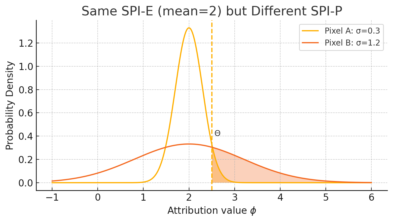
  Pixel	\(\mu\)	\(\sigma\)	SPI-E
  A	\(2.0\)	\(0.3\)	\(2.0\)
  B	\(2.0\)	\(1.2\)	\(2.0\)

  Although the two pixels share the same expected attribution (2.0), pixel B’s broader distribution lets it cross \(\Theta\) more often, so SPI-P marks B as “more likely to matter” while down-weighting A.

The Effect of the Base Distribution

In the Discussion (paper § 5), the authors point out that the Stick-Breaking Process (SBP) in the paper is instantiated with a uniform base distribution \(H = U(0,1)\) . Consequently, the expected path distribution \(G\) also becomes uniform, and the average path coincides with the straight-line IG path.

As future work, they propose replacing \(H\) with other distributions—e.g., a Gaussian—to steer the path so that it “moves more in the early steps or the late steps,” depending on the Gaussian mean.

The mechanism is easy to see from the path definition

\[\displaystyle \gamma_i(t) = \bar{x}_i + F_G(t)\bigl(x_i - \bar{x}_i\bigr), \qquad \frac{d\gamma_i}{dt} = G(t)\bigl(x_i - \bar{x}_i\bigr),\]

where \(F_G\) is the CDF and \(G\) is its PDF.

Whenever \(G(t)\) is large—that is, where the CDF is steep—the coordinate advances quickly; where \(G(t)\) is small, the path “idles.”

Now compare the CDF of the uniform distribution with CDFs of Gaussian distributions whose means differ:

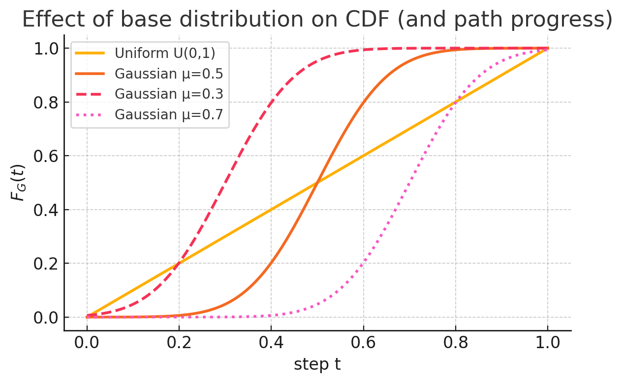
Base \(H\)	CDF \(F_G(t)\) shape	PMF/PDF \(G(t)\) slope	Path progress characteristics
Uniform \(U(0,1)\)	Linear	Constant	Constant speed — IG straight path
Gaussian \(\mu=0.5\) (symmetric)	S-curve	Large slope at middle ( \(t \approx 0.5\) ), small at both ends	Stagnant in early/late stages, fast in the middle
Gaussian \(\mu=0.3\) (left-shifted)	S-curve shifted left	Large slope in early part	Movement concentrated in early stage
Gaussian \(\mu=0.7\) (right-shifted)	S-curve shifted right	Large slope in later part	Movement concentrated in later stage

Because the PDF is the derivative of the CDF, changing the Gaussian mean changes where the PDF is steepest and therefore where \(F_G(t)\) rises most sharply.

Wherever the PDF is large (i.e. the CDF’s slope is high), the path advances rapidly; where it is small, progress is slow.

This illustrates why selecting Gaussian base distributions with different means lets us steer the path toward faster motion early, in the middle, or late in the integration interval.

Source

• BibTeX:

    @inproceedings{jeon2023beyond,
      title={Beyond Single Path Integrated Gradients for Reliable Input Attribution via Randomized Path Sampling},
      author={Jeon, Giyoung and Jeong, Haedong and Choi, Jaesik},
      booktitle={Proceedings of the IEEE/CVF International Conference on Computer Vision},
      pages={2052--2061},
      year={2023}
    }
  

• URL: https://openaccess.thecvf.com/content/ICCV2023/papers/Jeon_Beyond_Single_Path_Integrated_Gradients_for_Reliable_Input_Attribution_via_ICCV_2023_paper.pdf